Comparing three classic 1D search methods
Minimizer? I hardly know her!
What are we doing?
Finding a minimizer is a deceptively simple goal: we want the point where a function bottoms‑out. Getting to that point can be wildly different depending on the algorithm we choose. In this post, I revisit three classic one‑dimensional search methods—quadratic approximation, fixed‑step gradient descent, and backtracking (Armijo) line search, and pit them against the same trio of textbook functions.
My aim is two‑fold:
- Accuracy – Does the algorithm land on (or close to) the true minimizer?
- Efficiency – How many iterations does it take to get there?
(All functions come from Antoniou & Lu, Practical Optimization, Page 115, exercises 4.2-4.6.)
The Three Contestants
| Label | Function | Starting point |
|---|---|---|
| f₁ | ||
| f₂ | (domain ) | |
| f₃ |
Quadratic Approximation
A single Taylor expansion anchors the entire search. At a chosen point we evaluate the function, its gradient, and its Hessian matrix:
Those three numbers pin down a local quadratic model
whose stationary point is
[fcoef, tstat] = quadapprox(fgh1, t1);Upshot: Incredibly quick, but if the initial point is poorly chosen or the function is far from quadratic, the resulting accuracy suffers.
Fixed‑Step Gradient Descent
Classic steepest descent with a constant step size (here of the bracket width). Each update is
[tmin, fmin, ix] = steepfixed(fg1, t0, s);A small stepsize keeps things safe, but the cost is speed. A large stepsize risks a ping-pong around the minimizer.
Backtracking (Armijo) Line Search
Start with a generous step ( of the bracket) and shrink it geometrically (, ) until Armijo’s condition holds:
[tmin, fmin, ix] = steepline(fg1, t0, s0, beta, alpha);Think of it as a smarter version of fixed‑step: it learns how far it can safely go.
Results
| Function | Method | t_est | f_est | Iterations | abs(f_est − f_true) |
|---|---|---|---|---|---|
| f1 | Quadratic | 0.679 | 8.953 | 3.804e+00 | |
| f1 | Fixed step | 0.241 | 5.148 | 32.0 | 1.264e‑10 |
| f1 | Backtracking | 0.241 | 5.148 | 9.0 | 8.382e‑11 |
| f2 | Quadratic | 9.830 | 4.776 | 3.570e+00 | |
| f2 | Fixed step | 8.624 | 1.205 | 597.0 | 6.859e‑09 |
| f2 | Backtracking | 8.624 | 1.205 | 58.0 | 4.066e‑09 |
| f3 | Quadratic | 6.566 | 19.257 | 2.653e+01 | |
| f3 | Fixed step | 2.706 | ‑7.274 | 34.0 | 6.462e‑10 |
| f3 | Backtracking | 2.706 | ‑7.274 | 6.0 | 5.833e‑10 |
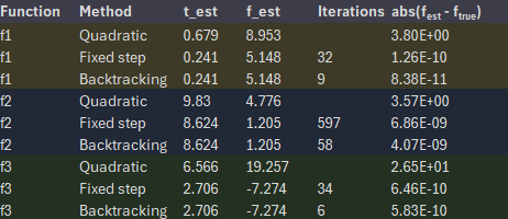
† Caveat: for f₃ the quadratic model returns the stationary point of the approximation, not the true minimizer (which is near ). The mismatch illustrates how brittle a single‑point quadratic fit can be on oscillatory functions.
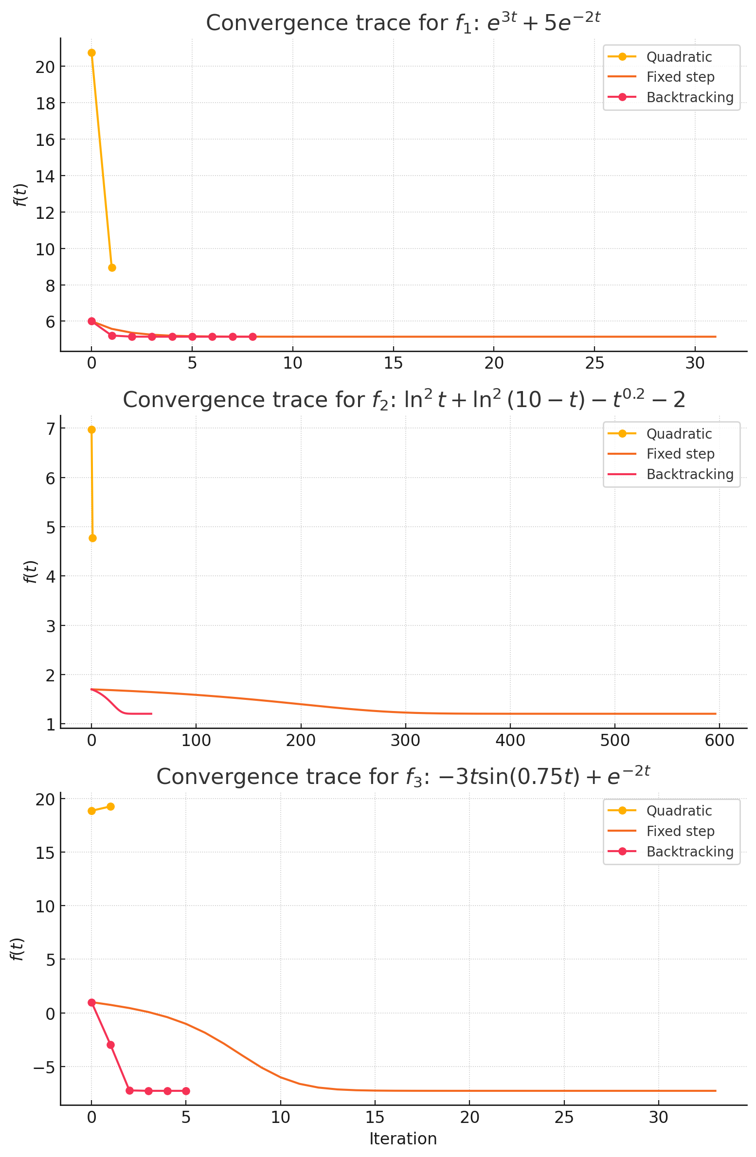
Graphs
Discussion
Quadratic Approximation is wildly quick. One shot and done, but it gambles on the curve really being quadratic nearby. On f₁ that gamble paid off reasonably; on f₃ it missed the valley altogether, highlighting it’s trade-off between speed and robustness.
Fixed‑Step descent was more accurate, but had a much worse iteration count (500 steps on f₂!). A fixed stepsize struggles to balance cautiousness and urgency across different situations.
Backtracking found the sweet spot. By dialing back the stepsize, whenever the Armijo test failed, it kept the gradient’s sense of direction while having an incredibly low stepsize. The result: same accuracy as fixed‑step in a fraction of the iterations.
TL:DR?
Every algorithm is a negotiation between prior assumptions and empirical feedback. Quadratic approximation assumes “I know the curvature.” Fixed‑step assumes “One size fits all.” Backtracking adapts iteratively.
Check out some MATLAB
% Objective & gradient for f1
f1 = @(t) exp(3*t) + 5*exp(-2*t);
g1 = @(t) 3*exp(3*t) - 10*exp(-2*t);

% Backtracking parameters
s0   = (1 - 0)*0.1;  % 1/10 of bracket width
beta = 0.5;
alpha= 0.5;
[tmin,fmin,ix] = steepline(@(t)deal(f1(t),g1(t)), 0, s0, beta, alpha);
Conclusion
In this small‑scale comparison test, backtracking line search emerged as the most balanced method, since it was accurate, yet economical. Fixed‑step is reasonably dependable when runtime is cheap. Quadratic approximation is a thrilling sprinter that sometimes dashes the wrong way.
The lesson that I can gain from this is that context matters. It’s easy to get stuck in a rut with a problem, using one strategy that feels ‘normal’ even if it’s not working. The key is just stepping back. Try coming at it from new angles and you’ll feel the trade-offs. One way might be clearer, but exhausting. Another might be easy, but messy. After a while, you stop trying to swim upstream and just let the problem’s own shape show you the way to the answer that clicks.
References
- Antoniou, A., & Lu, W.‑S. (2007). Practical Optimization. Springer.
- Ellis, R. E. Non‑Linear Data Analytics – Class Notes 2–4 (2025 edition).