Lasso Regression + Gaussian SVM: clean signals from small, messy data

What’s the situation?

We’re looking at a small but messy dataset while asking two questions: first, can Lasso regression (with 5-fold cross-validation) identify the few features that actually matter while performing about as well as an OLS baseline? Second, after reducing dimensionality with SVD to make the data viewable in two dimensions, can a Gaussian (RBF) SVM draw a clean decision boundary between two classes? The point is to keep the workflow simple, interpretable, and visual, so that the conclusions are easy to understand and act on.

The information and data derive from a class project to understand commodity data to track for hedging.

Why should we care?

Small datasets tend to have many variables, be a bit noisy, and be incomplete at times. Lasso shrinks unhelpful coefficients to zero, leaving us a compact model that can still be competitive with OLS. the SVD → SVM step gives a flexible nonlinear boundary in a visible space, which lets us perform a sanity check. Our sanity check states: if the separation is clean in two dimensions, we can trust our labels and our modeling choices. The combination gives clear signals, quick iteration, and visuals which can help us explain our results without an ungodly amount of math.

---

Equation List

Speaking of an ungodly amount of math, here’s my list of equations

OLS baseline

$$\min_{\beta}\ \lVert y - X\beta\rVert_2^2$$

Lasso (penalized form)

$$\min_{\beta}\ \frac{1}{2n}\,\lVert y - X\beta\rVert_2^2 \;+\; \lambda\,\lVert \beta\rVert_1$$

(equivalent constrained form)

$$\min_{\beta}\ \lVert y - X\beta\rVert_2^2 \quad \text{s.t.} \quad \lVert \beta\rVert_1 \le \theta$$

K-fold cross-validation objective (choose $\lambda$)

$$\mathrm{CV}(\lambda) =\frac{1}{K}\sum_{k=1}^{K}\frac{1}{n_k} \sum_{i\in \mathcal{I}_k}\bigl(y_i-\hat y^{(-k)}_i(\lambda)\bigr)^2$$

SVD and 2D projection (scores)

$$X = U\Sigma V^\top, \qquad Z = U_{[:,1:2]}\,\Sigma_{1:2,1:2} \quad (\text{equivalently } Z = X\,V_{[:,1:2]})$$

Gaussian (RBF) kernel

$$k(\mathbf{z},\mathbf{z}') \;=\; \exp\!\big(-\gamma \,\lVert \mathbf{z}-\mathbf{z}'\rVert_2^2\big) \;=\; \exp\!\left(-\frac{\lVert \mathbf{z}-\mathbf{z}'\rVert_2^2}{2\sigma^2}\right), \qquad \gamma \;=\; \frac{1}{2\sigma^2}.$$

MATLAB note: fitcsvm(...,'KernelFunction','rbf','KernelScale',σ) uses

$$k(\mathbf{z},\mathbf{z}')=\exp\!\big(-\lVert \mathbf{z}-\mathbf{z}'\rVert_2^2/(2\sigma^2)\big).$$

to match

$$\gamma = 1$$

in

$$\exp(-\gamma \lVert \mathbf{z}-\mathbf{z}'\rVert_2^2)$$

set

$$\sigma \;=\; \frac{1}{\sqrt{2}} \;\Longrightarrow\; \texttt{KernelScale} \;=\; \frac{1}{\sqrt{2}} \;\approx\; 0.7071 \, .$$

SVM decision function (for completeness)

$$\hat y(z) = \operatorname{sign}\!\left(\sum_{i=1}^{n}\alpha_i\,y_i\,k(z, z_i) + b\right)$$

---

Methodology

I prepared my data in three ways to handle the missing entries:

• Median imputation (robust to outliers)
• Mean imputation (great with uniform data, becomes risky with the introduction of extreme values)
• Row deletion (risky, but viable in small amounts)

With each version, I fit an OLS baseline and then ran Lasso with 5-fold cross-validation to select λ. The Lasso path (coefficient traces) and the CV error curve tell the story of sparsity versus fit.

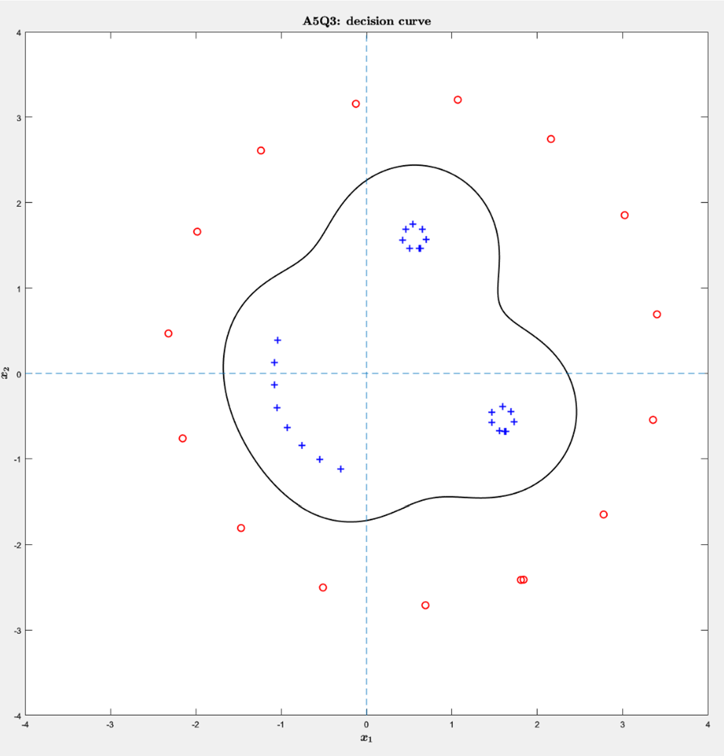
For classification, I standardized the imputed matrix. The 5D data were projected to 2D with SVD, and scaled x10 for display. After this, I trained an SVM with a Gaussian kernel (KernelScale = 10/sqrt(2), BoxConstraint = 1). The 2D setup lets us plot both the points and the zero-level decision contour to visually confirm separation.

Below is some MATLAB code to represent my methodology

% Median imputation (column-wise)
Xm = X;
for j = 1:size(X,2)
    col = Xm(:,j);
    mask = ~isnan(col);
    if any(mask)
        m = median(col(mask));
        col(~mask) = m;
    else
        col(:) = 0;  % or error('All-NaN column %d', j);
    end
    Xm(:,j) = col;
end

% Ensure y is a column
y = y(:);

% OLS baseline
beta_ols = Xm \ y;

% Lasso + 5-fold CV (lasso standardizes internally by default)
[B, FitInfo] = lasso(Xm, y, 'CV', 5);
beta_lasso = B(:, FitInfo.IndexMinMSE);
selected = find(beta_lasso ~= 0);

% Standardize → SVD → 2D
Xmz = zscore(Xm);
[U,S,~] = svd(Xmz, 'econ');
Z2 = U(:,1:2) * S(1:2,1:2);       % unscaled training coordinates
Zplot = 10 * Z2;                  % display-only scaling

% RBF SVM with gamma = 1  ⇒  KernelScale = 10/sqrt(2)
model = fitcsvm(Z2, labels, 'KernelFunction','rbf', ...
                'KernelScale', 10/sqrt(2), 'BoxConstraint', 1);

pred = predict(model, Z2);        % resubstitution accuracy
acc  = mean(pred == labels);

---

Results

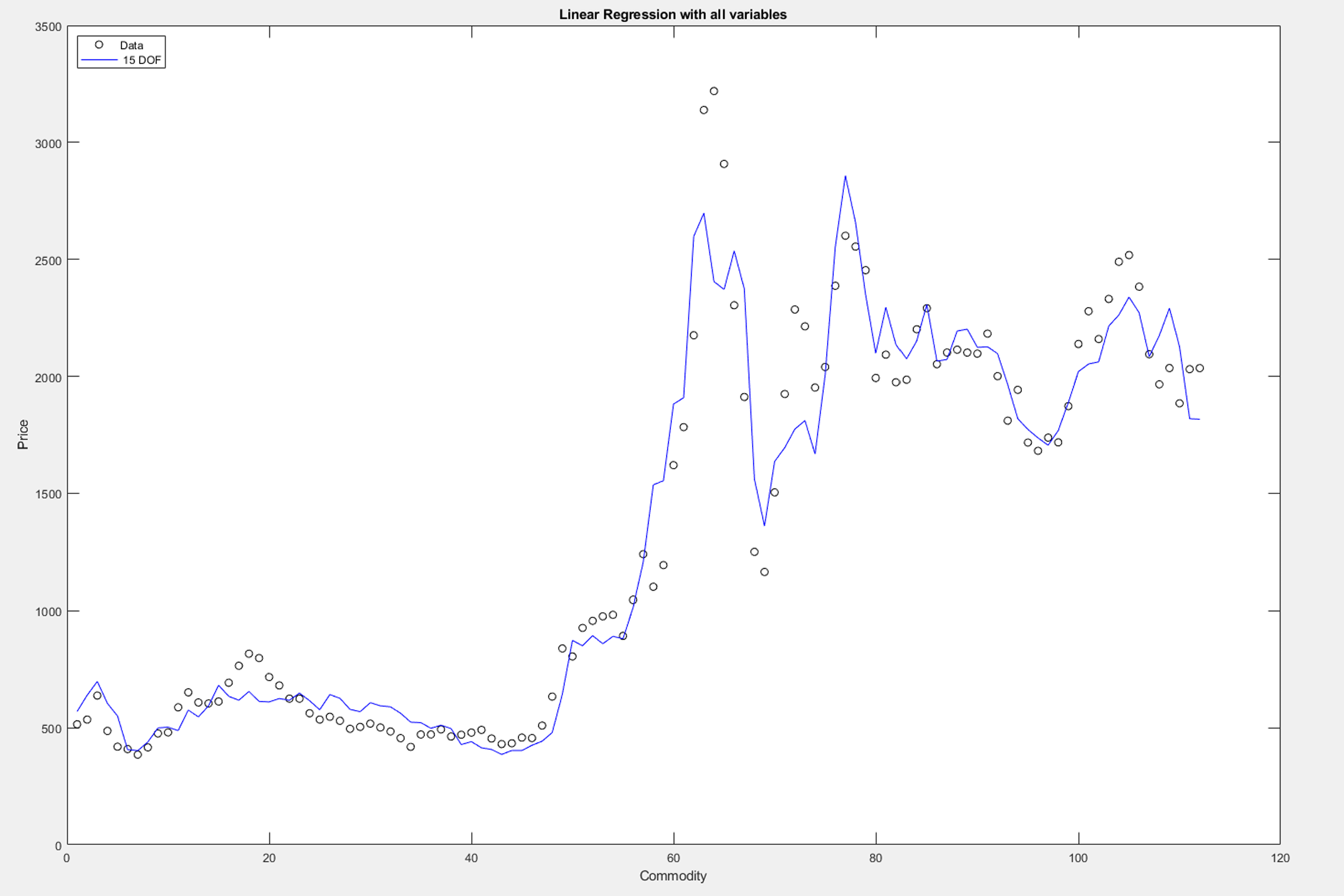
Regression

OLS hugged the data closely and gave us a solid reference line.

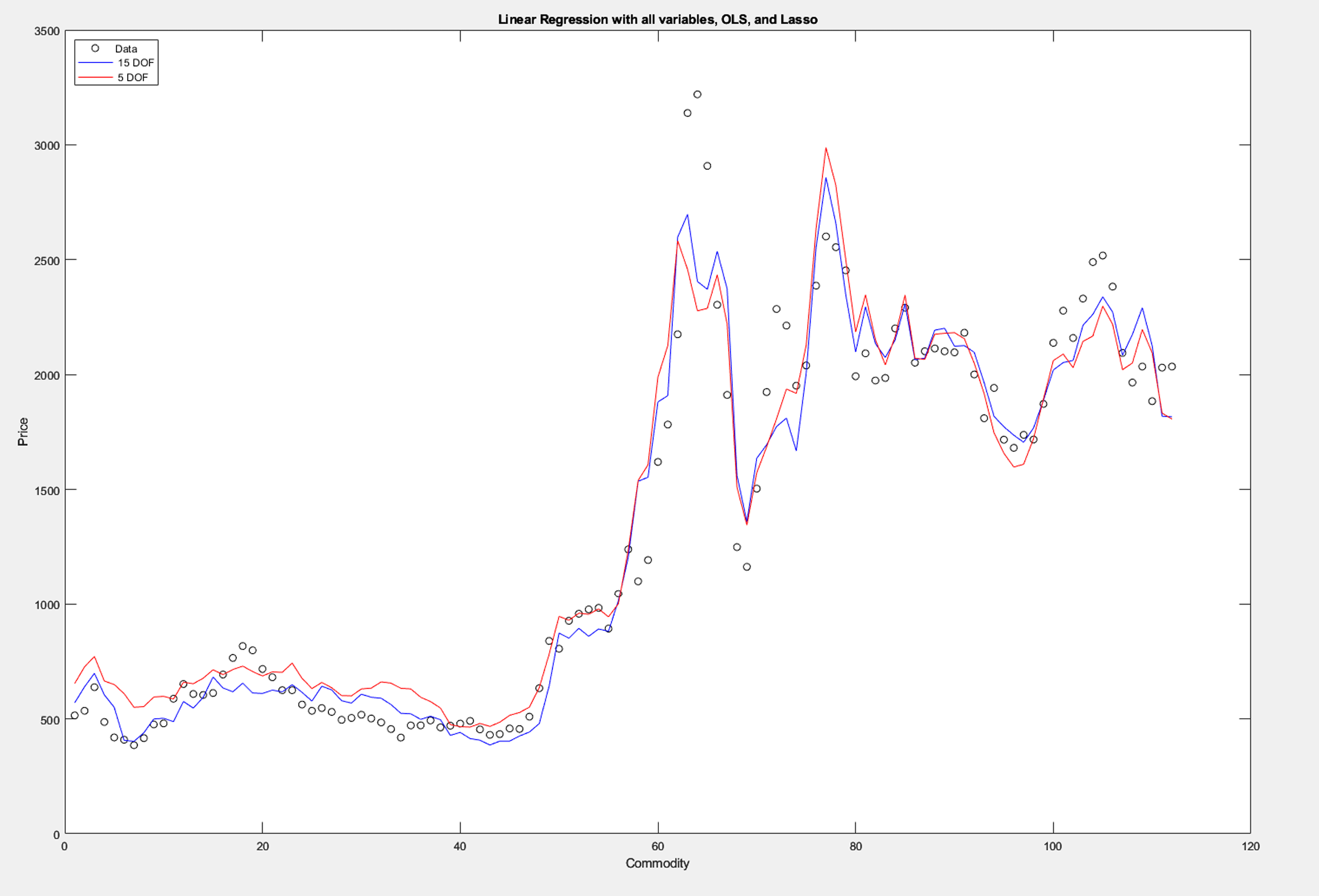
Lasso

Tuned by cross-validation, landed on a sparse location that was essentially indistinguishable from OLS in fit quality but relied on only five out of fifteen of the original variables.

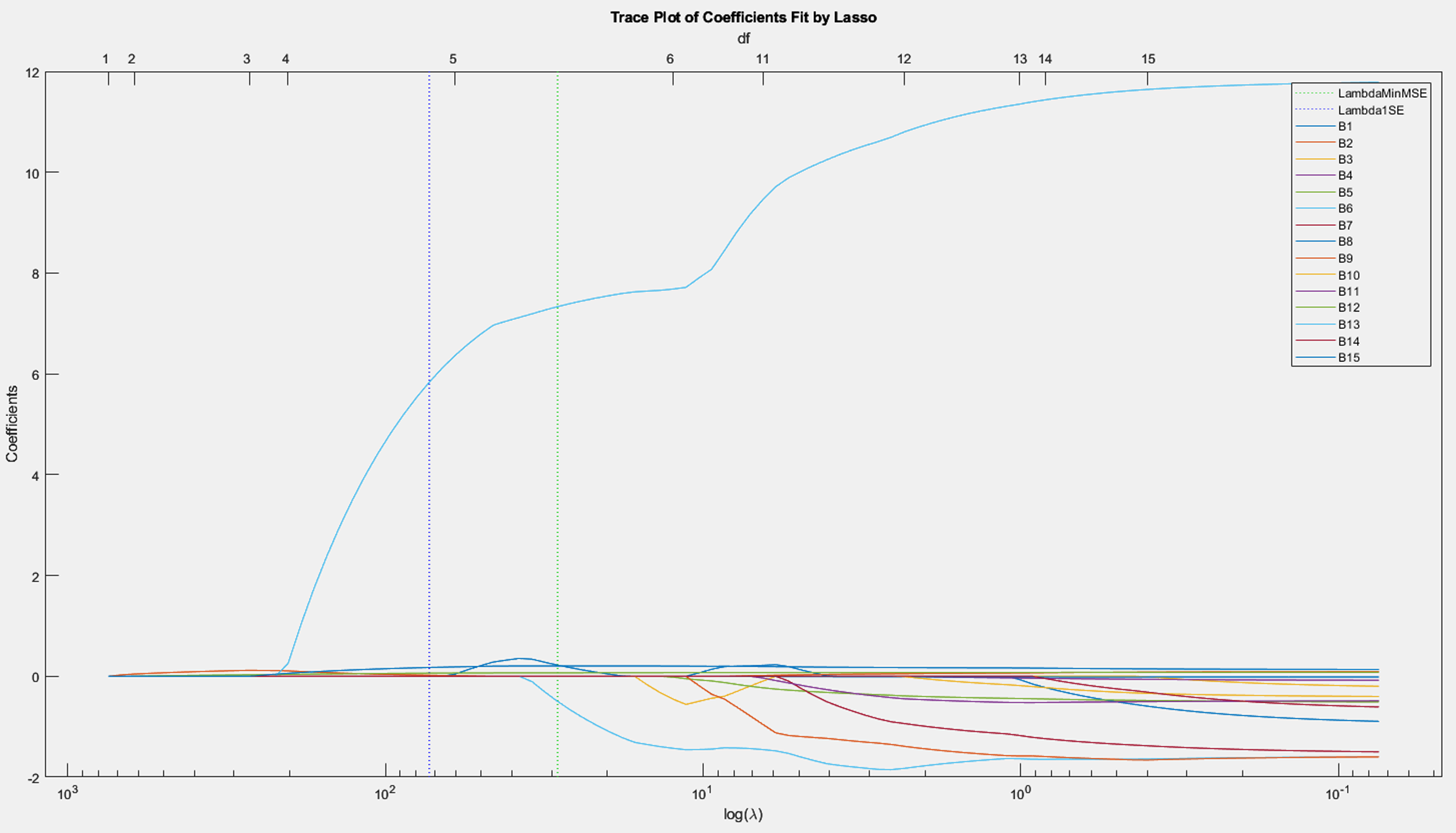
Trace plot

Here, one coefficient grew quickly while the rest hovered near zero until the constraint loosened. That would be clear evidence of a dominant signal.

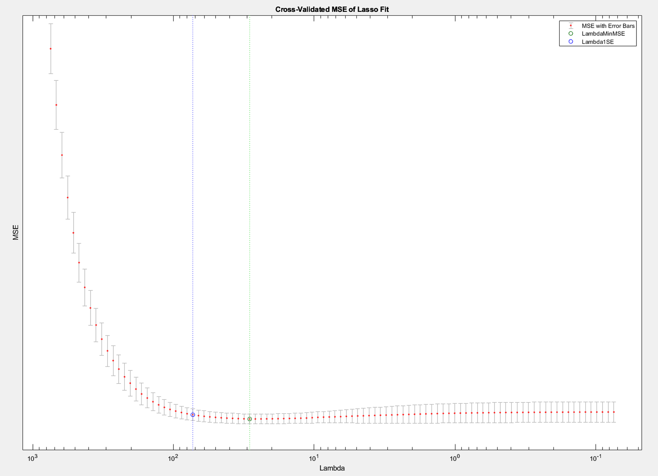
CV Curve

The CV curve narrowed the choice of the λ and confirmed that we didn’t need to turn on many coefficients to minimize error.

When we overlaid the final Lasso regression against the OLS line, the two curves tracked each other so closely that the practical difference was minimal while the interpretation was much cleaner.

On the topic of classification, the 2D SVD view showed two well-behaved groups. Training an RBF SVM on those coordinates produced a clean decision contour and achieved a correctness score of 100% on this dataset. The zero-level boundary wrapped the negative class and held the positives outside. There were no obvious anomalies and no mislabeled points.

---

A little discussion

Lasso delivered interpretability without sacrificing fit, which is what we want when working with a small dataset with many predictors. The missing-data choices (median vs. mean vs. deletion) led to the same conclusion, since only a small fraction of data was actually missing. Median is a safe default when outliers might exist, while deletion should only really be used for cases like the one here, where very little would be dropped. The 2D visualization with an RBF SVM doubled as a diagnostic: perfect separation in the plot matched the perfect score and suggested the labels were consistent. For deployment, you’d tune KernelScale and BoxConstraint via cross‑validation, but the takeaway stands: this pipeline is simple, interpretable, and effective.

---

The real world

In practice, this setup works well for signal screening and monitoring (pick a handful of drivers), quick anomaly checks (separation in 2D or flag overlap), and early-stage prototyping where you require defensible, explainable results fast. Lasso keeps regression lean and explainable, while the SVD → RBF SVM step gives you a high‑leverage visualization and a strong nonlinear classifier in small‑label regimes.

So where can we really apply this?

Here are some real world examples where this information comes useful:

Portfolio signals & risk regimes: When you have many macro indicators but limited history, we can use Lasso to parse it down to a small set of drivers that you can actually monitor. On the 2D SVD view, an RBF SVM separates “calm” vs “stess” regimes so you can approach with a reaction, rather than just a guess. Our practical move here is if the SVM decision score (margin) drops below 0 or within a small band ε of the boundary for a full week, tighten hedges. Also notify if and or when Lasso-selected indicator deviates > 2σ from its 30-day mean.

Manufacturing QA with small lots: You’re presented with few labeled units, many sensor channels. Lasso keeps only sensors that matter, and the 2D boundary gives a visual pass/fail envelope.

Predictive maintenance on sparse telemetry: Intermittent data feeds and missing values. Median imputation stabilizes input. Lasso identifies the handful of predictive counters, SVM separates “healthy” vs “degrading.” Let’s say the margin indicates “degrading” for N = 3 consecutive intervals, or the Lasso model’s residual jumps >3σ above its rolling baseline, it’s time to schedule maintenance.

Supply chain anomaly screening: Many potential drivers, messy demand. Lasso highlights a slim set of signals; SVM separates “expected” vs “disrupted” states.

---

References

Ellis, R. CISC 371 @ Queen’s University

MathWorks Documentation: lasso and fitcsvm function references.